LeNet-5 CNN
LeNet-5 is a convolutional neural network (CNN) architecture proposed by Yann
LeCun in 1998 for optical character recognition (handwritten digits). It is one
of the first CNNs to be successfully applied. It can be found in section 2 of
the paper LeCun1998.
You can find my annotated copy of the paper here.
Refer to only section 2 for the LeNet-5 model, as the paper proposes many more
things. The API code documentation can be found at mlhub.lenet.
The model implemented here consists of the following (just like many AI models):
Model: Original LeNet-5 architecture proposed in the paper
Data: The MNIST dataset from Yann LeCun’s Blog containing annotated/labelled digits for training and testing
Optimizer: The paper proposes an LM optimizer. The Stochastic Gradient Descent optimizer is used here (since it comes with PyTorch).
Loss: The same RBF (Radial Basis Function) output loss with MAP (maximum a posteriori) penalty term.
These are further described below. See the paper for more details.
Model
The architecture for LeNet-5 is shown below
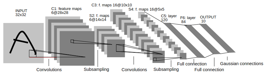
The layers are defined below
Input layer: The input is a
(32, 32)grayscale image that is mean normalized (the mean is 0 and standard deviation is 1 approximately).C1 convolution layer is a simple 2D Convolution layer with 1 input channel (from the input layer), 6 output channels, and a
(5, 5)kernel size (with stride 1). The output of this layer is of shape(6, 28, 28).S2 sub-sampling layer: Average the numbers, multiply with a trainable weight, and add a bias for each channel (of input). This is like average pooling but there is a weight multiplication and a bias offset (the weight and the bias are learnable parameters). This is implemented as standard convolution with weights as ones and stride as the kernel size. The result is multiplied with a trainable parameter, added with another. The sub-sampling is implemented as the
SubSamplingLayerclass. The input and output of this layer are of shape(6, 14, 14).C3 custom convolution layer: This is like the same convolution layer (like C1), but the weights of some input channels are masked off (set zero) so that not every input channel is connected to every output channel (the kernel has a specific connectivity map). The output of this layer is of shape
(16, 10, 10).S4 is another sub-sampling layer like S1. The output of this layer is of shape
(16, 5, 5).C5 is a convolution layer like C1. The output of this layer is of shape
(120, 1, 1), which is flattened to120dimension vector.F6 is a linear layer with
84output units (dimension).Output layer is a radial basis function layer that outputs a
10dimensional vector (each element is for a digit - 0 through 9). The RBF is described in more detail below.
A sigmoid-like activation function is used in between the layers. It’s formulated as
This activation function is implemented as SigmoidSquashingActivation.
The entire network is implemented in the LeNet5 class.
Custom Convolution Layer
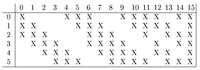
The connectivity map for layer C3, in Table 1 of the LeCun1998 paper.
The 6 rows in the above figure are for the 6 input channels and the 16 columns are for the 16 output channels. For example, the third output channel (column heading 2 in the figure) is connected with 3rd through 5th input channels only. The weights for other channels is set to zero (so they’re not connected).
The first six output channels are connected to sets of three consecutive input channels, next six outputs are with sets of four consecutive input channels, next three output channels are with sets of four disjoint input channels, and the last one is connected to all input channels (like in a normal convolution).
The reason for choosing this pattern, according to the paper, is to provide a
split and to prevent the network from learning symmetric (same) weights. This
is implemented as the CustomConvLayer class.
Radial Basis Function
A radial basis function is parameterized by weights \(w_{ij}\) (\(i\)
being [0, 9] and \(j\) being [0, 83]). It gets inputs \(x_j\)
and the output \(y_i\) (for the \(i^{th}\) output unit) is given by
This is basically the squared Euclidean distance from the weights. The weights
are not trainable and are a template. The weight values are +1 or -1.
The weights are made by the corresponding character representation on a
(7, 12) grid (+1 for black foreground and -1 for white background).
The weights are flattened to match the 84 dimensional input shape.
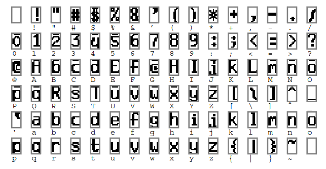
The initial template parameters (weights) of the RBF. We’re only interested in
digit characters 0 through 9. We can slide a (12, 7) grid and fill in the
template/weight values. From Figure 3 of the
LeCun1998 paper.
The output \(y_i\) with the least value is the predicted digit. This is
implemented as the RBFUnits class.
Data
We use the digits MNIST dataset that contains size normalized handwritten
characters. There are 60,000 digits for training and 10,000 digits for
testing. Since there’s isn’t a separate validation set, we’ll use the test set
as the validation set (this is unconventional). We do not use any distortions
for data augmentation when training. The entire dataset can be found on this
website: http://yann.lecun.com/exdb/mnist/.
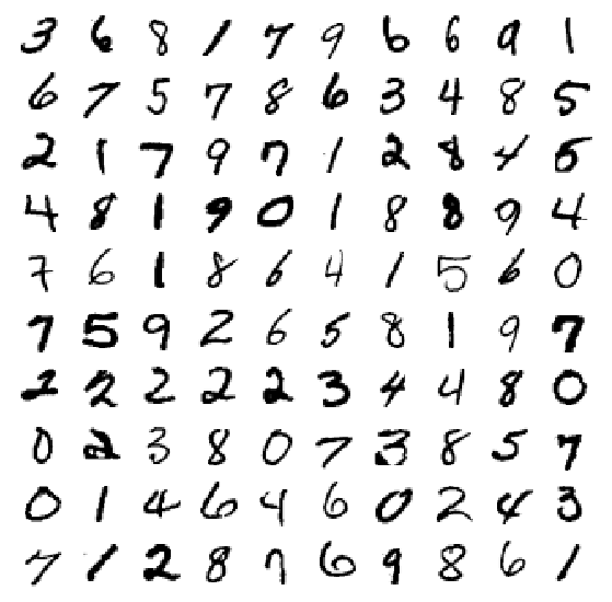
Some handwritten examples from the MNIST dataset.
The dataset for this is implemented in the MNISTDataset class.
Loss
The training loss for this method is the MAP (maximum a posteriori) criterion. This means that in addition to pushing down the penalty of correct class (like the MSE criterion - the output of the RBF), this also pulls up the penalties of incorrect classes. The loss is formulated as follows
The above is Equation 9 of the LeCun1998 paper. Where \(W\) are the trainable parameters (weights) of the network, \(P\) is the training batch size, \(Z^p\) is an input sample from the batch, \(D^p\) is the label of the input sample, and \(j\) is a small positive number.
The first term \(y_{D^p} \left ( Z^p, W \right )\) is the RBF output of the
unit \(D^p\) (correct output sample). We ideally want this to be zero since
the output of the RBF unit is the Euclidean distance from template (when the
input to RBF matches the template, it should output 0).
The second term (containing the \(log\) function) is to make all RBF units output some value (so that they do not collapse to the trivial solution of outputting all zeros). The higher the \(y_i\) value, the lower is the \(e^{-y_i}\) value (and the lower is the loss).
The two terms ensure that the correct label is pushed down (lower value output)
and the incorrect label is pushed up (higher value output). This is implemented
in the TrainingLoss class.
Training
The model was trained for 50 epochs using the SGD optimizer with learning rate 0.01
and the model checkpoint for the lowest test error was saved (2.34 % error
on MNIST test set).
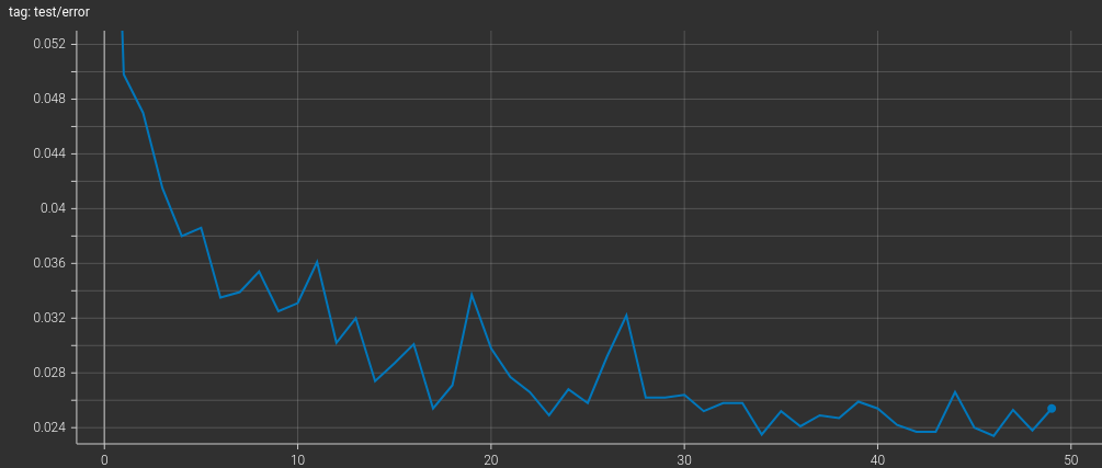
The training curve showing test error decreasing with each epoch. It becomes nearly stagnant after a few epochs.
Ideally, there is a separate validation set for selecting the best model. We use
the test split here.
See the mlhub.lenet.train module for more information on the API.
Results
References
The following are great resources for learning about CNNs